What is deep learning?
What is deep learning?
1.1 Artificial intelligence, machine learning, and deep learning
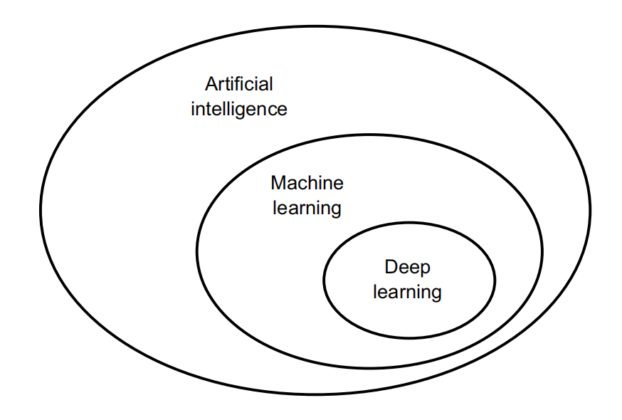
1.1.1Artificial intelligence

For a fairly long time, most experts believed that human-level artificial intelligence could be achieved by having
programmers handcraft a sufficiently large set of explicit rules for manipulating knowledge stored in explicit databases. This approach is known as symbolic AI.
Symbolic AI proved suitable to solve well-defined,logical problems,such as playing chess, it turned out to be intractable to figure out explicit rules for solving more complex, fuzzy problems, such as image classification, speech recognition, or natural language translation. A new approach arose to take symbolic AI’s place:machine learning.
1.1.2 Machine learning
Machine Learning looks at the input data and the corresponding answers,and figures out what the rules should be.
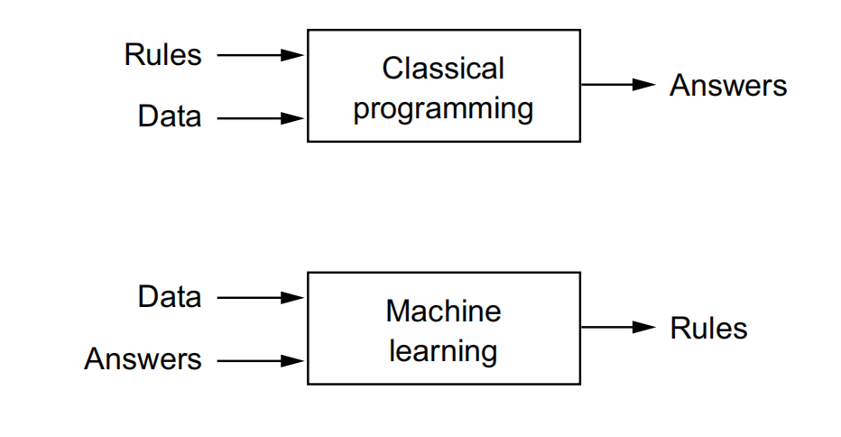
1.1.3 Learning rules and representations from data
To define deep learning and understand the difference between deep learning and other machine learning approaches, first we need some idea of what machine learning algorithms do. We just stated that machine learning discovers rules for executing a data processing task, given examples of what’s expected. So, to do machine learning, we need three things:
- Input data points—For instance, if the task is speech recognition, these data points could be sound files of people speaking. If the task is image tagging, they could be pictures.
- Examples of the expected output—In a speech-recognition task, these could be human-generated transcripts of sound files. In an image task, expected outputs could be tags such as “dog,” “cat,” and so on.
- A way to measure whether the algorithm is doing a good job—This is necessary in order to determine the distance between the algorithm’s current output and its expected output. The measurement is used as a feedback signal to adjust the way the algorithm works. This adjustment step is what we call learning
A machine learning model transforms its input data into meaningful outputs, a process that is “learned” from exposure to known examples of inputs and outputs. Therefore, the central problem in machine learning and deep learning is to meaningfully transform data: in other words, to learn useful representations of the input data at hand—representations that get us closer to the expected output.
What is representations?
At its core, it’s a different way to look at data—to represent or encode data.
Two different representations of a color image:
- RGB(red-green-blue)
- HSV(hue-saturation-value)
The task ‘select all red pixels in the image’ is simpler in the RGB format.
The task ‘make the image less saturated’ is simpler in the HSV format.
Machine learning models are all about finding appropriate representations for their input data—transformations of the data that make it more amenable to the task at hand.
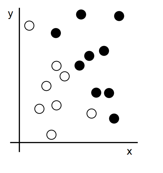
We have a few white points and a few black points. Let’s say we want to develop an algorithm that can take the coordinates (x, y) of a point and output whether that point is likely to be black or to be white.
Let’s say we want to develop an algorithm that can take the coordinates (x, y) of a point and output whether that point is likely to be black or to be white. In this case:
The inputs are the coordinates of our points.
The expected outputs are the colors of our points.
A way to measure whether our algorithm is doing a good job could be, for instance, the percentage of points that are being correctly classified.
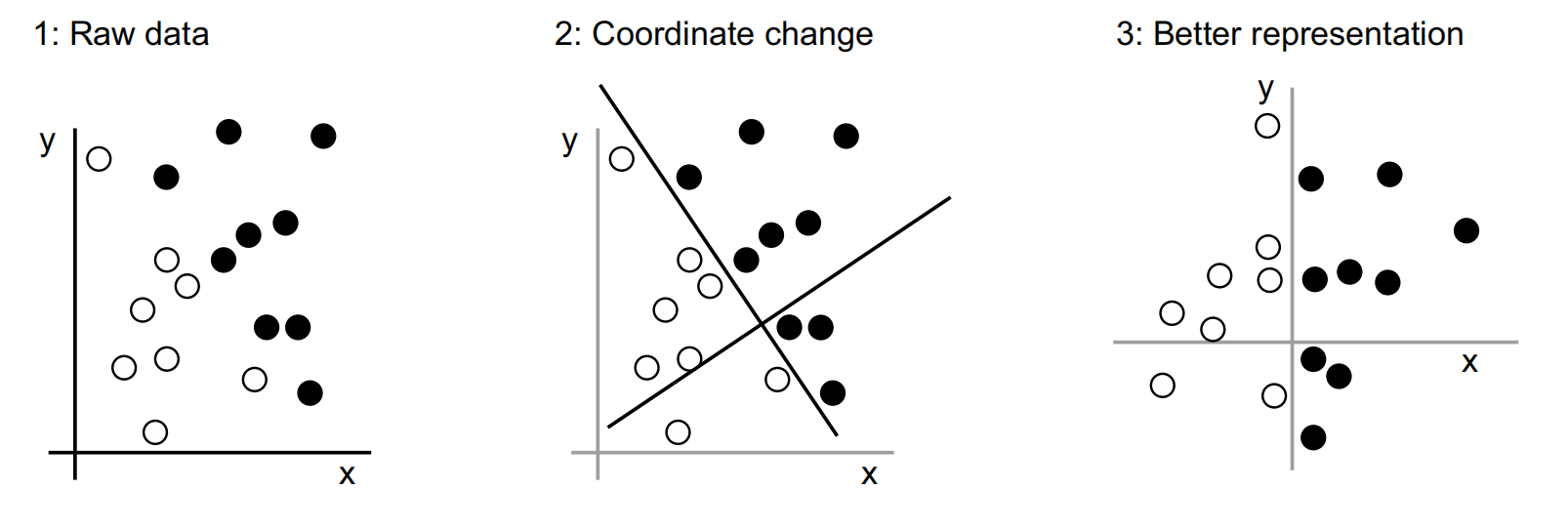
With this representation, the black/white classification problem can be expressed as a simple rule: “Black points are such that x > 0,” or “White points are such that x < 0.”
In this case we defined the coordinate change by hand.This is a simple problem.But,can we do the same if the task were to classify images of hand written digits?
This is possible to an extentt.But if you come across a new example that breaks your rules,you have to add a new transformation and new rules,while taking account their interaction with every previous rule.
The process is painful,then we try to find a way to automate it.What if we tried systematically searching for different sets of automatically generated representations of the data and rules based on them, identifying good ones by using as feedback the percentage of digits being correctly classified in some development dataset? We would then be doing machine learning. Learning, in the context of machine learning, describes an automatic search process for data transformations that produce useful representations of some data, guided by some feedback signal—representations that are amenable to simpler rules solving the task at hand.
These transformations contains coordinate changes, taking a histogram of pixels ,counting loops,linear projects, translations,nonlinear operations ,and so on.
Machine learning algorithms aren’t usually creative in finding these transformations;they’re merely searching through a predefined set of operations, called a hypothesis space. For instance, the space of all possible coordinate changes would be our hypothesis space in the 2D coordinates classification example.
So that’s what machine learning is, concisely: searching for useful representations and rules over some input data, within a predefined space of possibilities, using guidance from a feedback signal. This simple idea allows for solving a remarkably broad range of intellectual tasks, from speech recognition to autonomous driving.
1.1.4 The “deep” in “deep learning”
Deep learning is a specific subfield of machine learning: a new take on learning representations from data that puts an emphasis on learning successive layers of increasingly meaningful representations.
The “deep” in “deep learning” isn’t a reference to any kind of deeper understanding achieved by the approach; rather, it stands for this idea of successive layers of representations.
How many layers contribute to a model of the data is called the depth of the model. Other appropriate names for the field could have been layered representations learning or hierarchical representations learning. Modern deep learning often involves tens or even hundreds of successive layers of representations, and they’re all learned automatically from exposure to training
data.
Meanwhile, other approaches to machine learning tend to focus on learning only one or two layers of representations of the data (say, taking a pixel histogram and then applying a classification rule); hence, they’re sometimes called shallow learning
In deep learning, these layered representations are learned via models called neural networks, structured in literal layers stacked on top of each other.
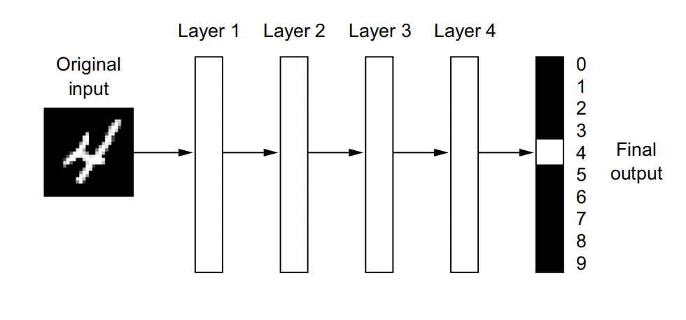
The network transforms the digit image into representations that are increasingly different from the original image and increasingly informative about the final result. You can think of a deep network as a multistage information distillation process, where information goes through successive filters and comes out increasingly purified (that is, useful with regard to some task).
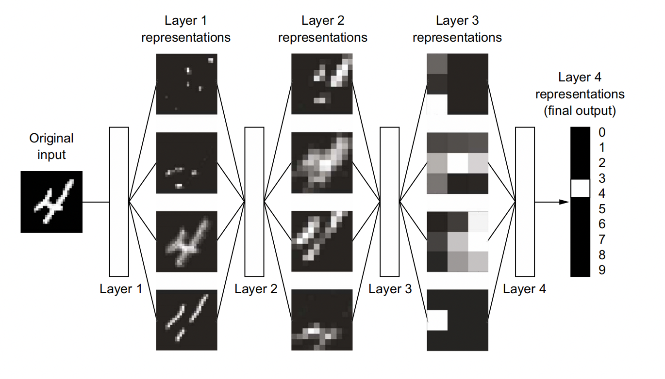
So that’s what deep learning is, technically: a multistage way to learn data representations.
1.1.5 Understanding how deep learning works, in three figures
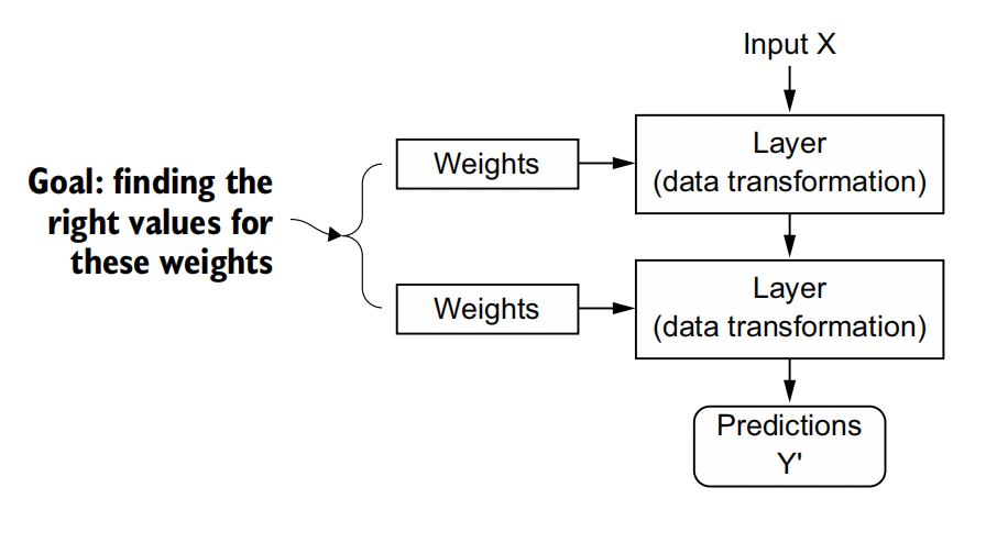
The specification of what a layer does to its input data is stored in the layer’s weights, which in essence are a bunch of numbers. In technical terms, we’d say that the
transformation implemented by a layer is parameterized by its weights .(Weights are also sometimes called the parameters of a layer.) In this context, learning means finding a set of values for the weights of all layers in a network, such that the network will correctly map example inputs to their associated targets.
But here’s the thing: a deep neural network can contain tens of millions of parameters. Finding the correct values for all of them may seem like a daunting task, especially given that modifying the value of one parameter will affect the behavior of all the others!
To control something, first you need to be able to observe it. To control the output of a neural network, you need to be able to measure how far this output is from what you expected. This is the job of the loss function of the network, also sometimes called the objective function or cost function. The loss function takes the predictions of the network and the true target (what you wanted the network to output) and computes a distance score, capturing how well the network has done on this specific example.
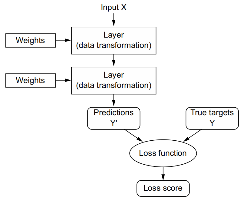
The fundamental trick in deep learning is to use this score as a feedback signal to adjust the value of the weights a little, in a direction that will lower the loss score for the current example . This adjustment is the job of the optimizer, which implements what’s called the Backpropagation algorithm: the central algorithm in deep learning.
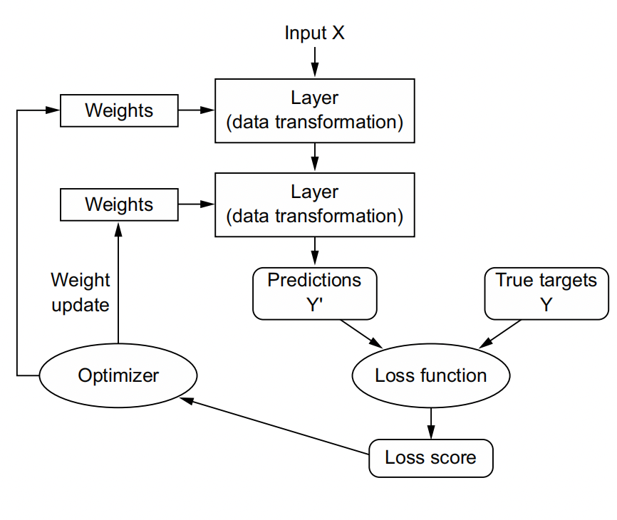
Initially, the weights of the network are assigned random values, so the network merely implements a series of random transformations. Naturally, its output is far from what it should ideally be, and the loss score is accordingly very high. But with every example the network processes, the weights are adjusted a little in the correct direction, and the loss score decreases. This is the training loop, which, repeated a sufficient number of times (typically tens of iterations over thousands of examples), yields weight values that minimize the loss function. A network with a minimal loss is one for which the outputs are as close as they can be to the targets: a trained network.
1.2 A brief history of machine learning
1.2.1 Probabilistic modeling
Probabilistic modeling is the application of the principles of statistics to data analysis. It is one of the earliest forms of machine learning, and it’s still widely used to this day. One of the best-known algorithms in this category is the Naive Bayes algorithm.
- Naive Bayes
- logistic regression
1.2.2 Early neural networks
The first successful practical application of neural nets came in 1989 from Bell Labs, when Yann LeCun combined the earlier ideas of convolutional neural networks and backpropagation, and applied them to the problem of classifying handwritten digits. The resulting network, dubbed LeNet, was used by the United States Postal Service in the 1990s to automate the reading of ZIP codes on mail envelopes.
1.2.3 Kernel methods
Kernel methods are a group of classification algorithms, the best known of which is the Support Vector Machine (SVM).
SVM is a classification algorithm that works by finding “decision boundaries” separating two classes.
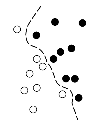
- The data is mapped to a new high-dimensional representation where the decision boundary can be expressed as a hyperplane.
- A good decision boundary (a separation hyperplane) is computed by trying to maximize the distance between the hyperplane and the closest data points from each class, a step called maximizing the margin. This allows the boundary to generalize well to new samples outside of the training dataset.
1.2.4 Decision trees, random forests, and gradient boosting machines
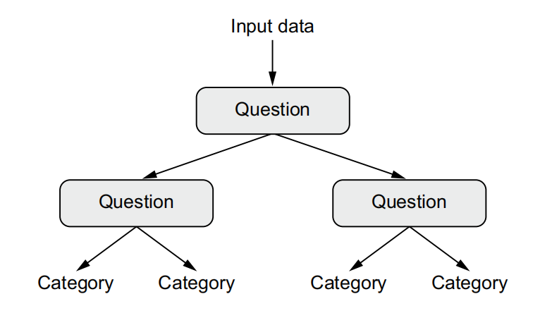
Decision trees are flowchart-like structures that let you classify input data points or predict output values given inputs.
In particular, the Random Forest algorithm introduced a robust, practical take on decision-tree learning that involves building a large number of specialized decision trees and then ensembling their outputs.